SEOs and Excel – they have chemistry. Despite being absolutely intimidating, Excel has something SEOs can’t resist: flexibility, extensive data manipulation capabilities, complex analysis options, numerous integrations, and offline access if needed.
If you’ve already fallen for Excel but need a helping hand to figure it out, here it is – 13 Excel formulas for managing SEO data.
Before you throw yourself into Excel formulas, I would like to remind you that SEO PowerSuite provides various SEO data that can be extracted and imported into Excel or Google Sheets for further analysis and management. Here are just a few things you can extract from each of our tools:
Rank Tracker
- Keywords and the URLs that rank for them
- Keyword difficulty scores
- SEO/PPC data: number of searches, estimated traffic, and CPC
- Keyword rankings and progress
- Google Search Console data: clicks, impressions, and CTR
- Google Analytics data: sessions and page bounce rates
Website Auditor
- HTTP status codes and page sizes
- Link data: outbound and inbound links, broken links, and click depth
- On-page elements: titles, meta descriptions, mapped keywords, optimization rates, word count
- Open graph and structured data markup elements
- Images with empty alt texts
SEO Spyglass
- Backlink pages and linked pages
- Domain and page inLink rank (PageRank analog)
- Dofollow/nofollow links and their anchor texts
- Prospective and intersecting domains
LinkAssistant
- Link prospect data: URLs, contact names and emails, and statuses
- Prospect’s domain traffic, inLink rank
To extract and import these data into Excel or Google Sheets, you can use the export feature in each tool and choose the format that best suits your needs (e.g., CSV, Excel).
Download SEO PowerSuite
Now let’s move to the Excel formulas themselves.
SUBSTITUTE – to replace specific text in a text string
Formula: =SUBSTITUTE(text, old_text, new_text, [instance_num])
SEO use cases:
- Cleaning up data. You can use the SUBSTITUTE formula when you need to remove unwanted characters or strings from your data. For instance, you can remove special characters or extra spaces from your web page titles or meta descriptions to make them neat and clean.
- Researching keywords. With the formula, you can modify your keywords and generate additional variations. For example, you can replace the letter "s" with "z" (like in analyse and analyze) to create a different spelling of a keyword or replace a prefix or suffix to generate long-tail keywords.
How-to:
- Select the cell where you want to display the result and enter the SUBSTITUTE formula in the cell.
- Inside the formula, first specify the text cell that you want to modify, then the old text that you want to replace, and finally the new text that you want to insert in its place. If it’s needed, you can specify the instance number – the occurrence of the old text you want to replace with the new one. For example, you can specify instance_num as 2, and only the second letter or word of the old text will be replaced with the new one.
- Press Enter to see the result.
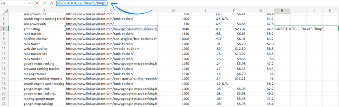
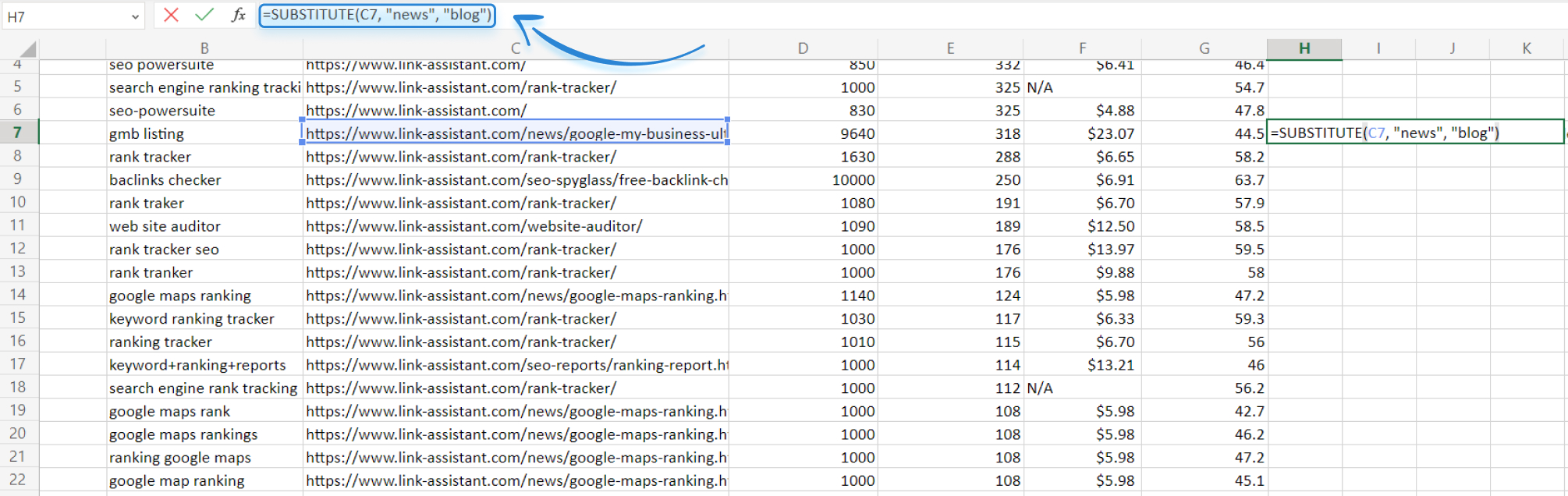
Here's an example. I'm moving my blog articles to the new folder "blog". Hence, I need to replace "news" in my URL with "blog". To do so, I enter =SUBSTITUTE(C7, "news", "blog")" in a separate cell of my spreadsheet, where C7 is the cell containing the original URL.
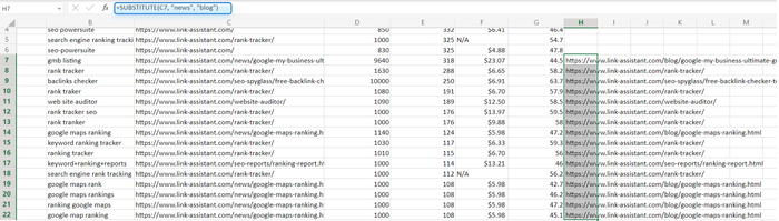
Later I can drag the formula across the whole column and it will replace the values for other text strings as well:
The rule of auto-filling will work with all the formulas unless you include absolute or mixed references into them.
Note
If for some reason your formulas don’t work, try using semicolons instead of commas in them. The reason for that lies in the regional difference in default list separators in the European (semicolon) and American (comma) countries.
Alternatively, you can go to the regional settings of your computer and set comma as a List Separator.
CONCATENATE – to combine the content of several cells
Formula: =CONCATENATE(text1, [text2], ...)
SEO use cases:
- Creating title tags. You can create optimized title tags for your web pages with CONCATENATE. For example, you can combine the main keyword, the brand name, and other relevant information to create title tags that are both informative and SEO-friendly.
- Researching keywords. If you have an ecommerce site with lots of products that differ by a set of variables (gender, color, rise, etc.), you may create all the needed combinations (male red t-shirt, female yellow t-shirt) much faster.
- Analyzing data. You may need to combine different data points into a single cell. For instance, you can combine the domain name, the page URL, and the page title into a single cell for easier analysis.
How-to:
- Select the cell where you want the result to appear and enter the =CONCATENATE formula in the cell.
- Inside the formula, specify the text strings that you want to combine, separated by commas.
- Press Enter to display the concatenated string.
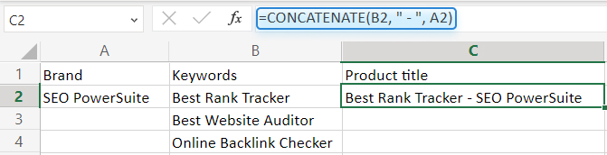
For example, I have a huge site with lots of similar pages and need to come up with titles for them. What I can do here is combine a page's main keyword phrase with a brand name into a single title tag. So, in my spreadsheet, I select the cell and enter "=CONCATENATE(B2, “ - “, A2). Here, B2 is the main keyword cell and A2 is the brand name cell.
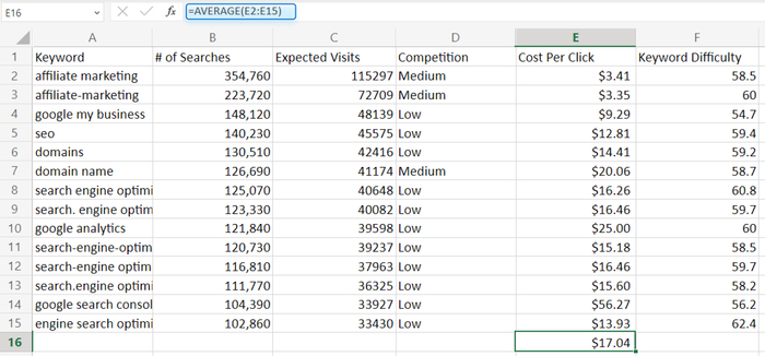
AVERAGE – to calculate the average of some metric
Syntax: =AVERAGE(number1, [number2], ...)
SEO use cases:
Basically, all the use cases of this formula boil down to one category – analyzing numerical data. With the formula, you can calculate the average:
- ranking of a group of keywords across multiple search engines or over time. This is needed to track your SEO progress and identify areas for improvement.
- domain authority, page authority, or other backlink metrics for a group of websites or web pages. By doing that, you identify high-quality backlink opportunities and monitor the effectiveness of your link-building efforts.
How-to:
- Select the cell and enter the =AVERAGE formula.
- Inside the formula, specify the needed range of cells and press Enter to calculate the data average.
For example, I want to calculate the average CPC for a group of keywords. So, I enter "=AVERAGE(F2:F15)" in a separate cell of my sheet, where F2:F15 is the range of cells I need to calculate the average for. After pressing Enter, I see the average CPC for those keywords.
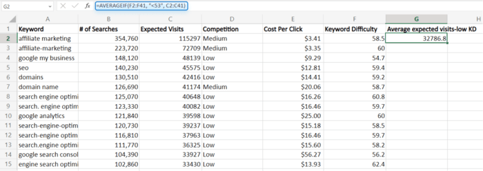
AVERAGEIF – calculate the average of a range based on a specified condition
Formula: =AVERAGEIF(range, criteria, [average_range])
SEO use cases:
In two words, use the formula for performance analysis. With it, you can calculate the average:
- page load time for a specific category of web pages, such as pages belonging to a particular folder or with specific tags. It can help you identify performance issues specific to certain sections of your site.
- ranking of keywords that meet specific criteria (keywords related to a specific product or keywords with a certain search volume range). This way, you can get insights into the performance of different keyword segments.
- backlink count for websites that satisfy certain conditions, like websites from a particular industry or websites with a specific domain authority range. With this info, you can easily analyze the backlink profiles of different websites.
How-to:
- Select the cells where you want the result to appear and enter the =AVERAGEIF formula in the cell.
- Inside the formula, specify the range of cells to evaluate and the condition to be met.
- Press Enter.
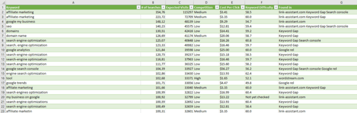
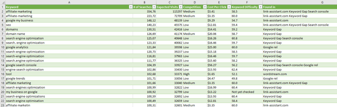
For example, I need to calculate the average expected visits for my low-difficulty keywords. In my spreadsheet, I select the needed cell and enter "=AVERAGEIF(F2:F41, "<53", C2:C41)". F2:F41 is the range that I will set the condition for and C2:C41 are the actual cells to be used to find the average.
Note
Use AVERAGEIFS if you need to calculate the average of all cells that meet multiple criteria. The syntax will be the following: =AVERAGEIFS(average_range, criteria_range1, criteria1, [criteria_range2, criteria2], ...)
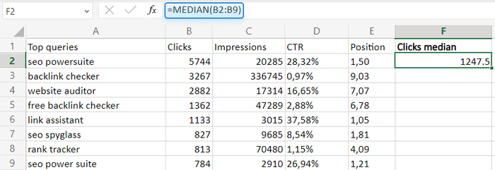
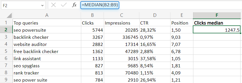
Formula: =MEDIAN(number1, [number2], …)
SEO use cases:
- Analyzing rankings. You can calculate the median ranking position of a group of keywords.
- Analyzing traffic. You can determine the median organic traffic volume for a set of landing pages. This way, you can understand the typical traffic level and identify pages with unusually high or low performance.
How-to:
- Select the cell and enter the =MEDIAN formula.
- Inside the formula, specify the range of cells you want to find the median of.
- Press Enter.
For example, I want to calculate the median number of clicks for a group of keywords. So, I select the cell where I want the result to appear and enter "=MEDIAN(B2:B9)". Here, B2:B9 is the range of cells you want to find the median of.
Side note: Difference between AVERAGE and MEDIAN functions
This may confuse you if you know little about these two functions. The best way to explain the difference is to show the difference:
LEN – to check the length of your text data
Formula: =LEN(text)
SEO use cases:
The LEN function can be useful for text data analysis. You can calculate the length:
- of URLs for a group of web pages to identify excessively long URLs, which can negatively impact SEO.
- of meta titles and descriptions for a group of web pages. This can help you ensure that your meta tags are within the optimal length limits for search engines.
- of your target keywords to spot long-tail keywords to optimize for.
How-to:
- Select the cell where you want to display the result and enter the LEN formula in the cell.
- Inside the formula, specify the cell or range of cells containing the text you want to analyze.
- Press Enter to calculate the length of the text.
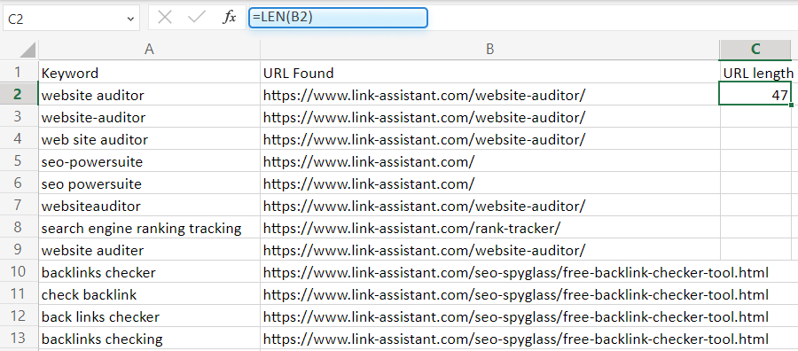
For example, I need to calculate the length of the URL for a specific web page. I enter "=LEN(B2)" in a separate cell, where B2 is the cell containing the URL. I press Enter and see the result.
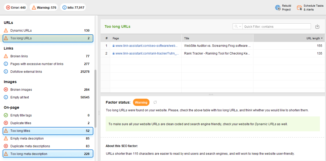
FYI: WebSite Auditor detects too long URLs, titles, and descriptions on your site
To access the report, go to Site Structure > Site Audit and scroll down to the URLs and On-page sections:
Download WebSite Auditor
Formula: =IF(logical_test, [value_if_true], [value_if_false])
SEO use cases:
- Analyzing keyword rankings. You can analyze keyword rankings across different search engines or time periods. For example, you can compare a keyword's current ranking to its ranking in the previous month and get the formula to display a message if the ranking has improved or not.
- Analyzing backlinks. You can analyze backlink metrics and identify potential issues or opportunities. For example, you can check whether a backlink comes from a high-quality site.
How-to:
- Select the cell and enter the IF formula.
- Inside the formula, specify the logical test that you want to apply. This can be a comparison between two values, or a condition based on a certain criterion.
- Specify the value that should be displayed if the logical test is true, and the value that should be displayed if the logical test is false.
- Press Enter to display the result.
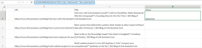
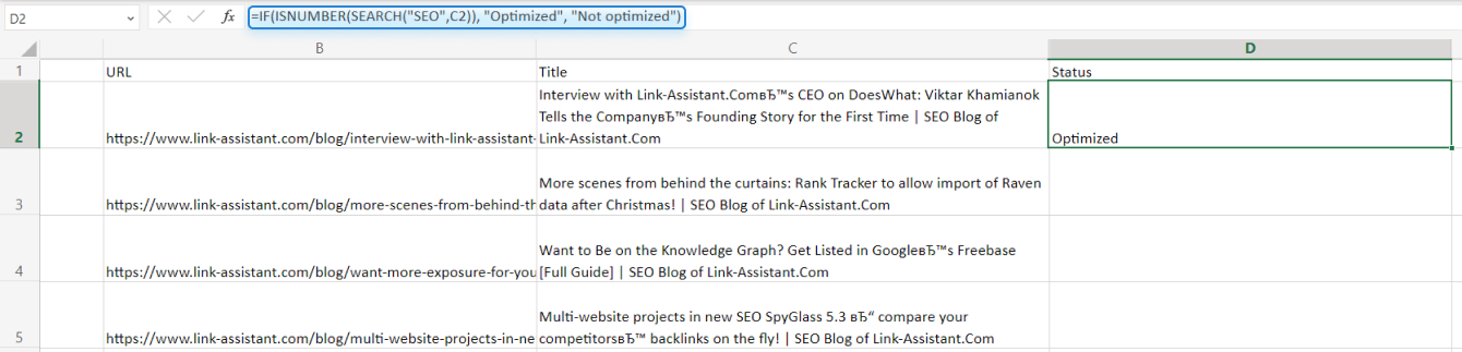
For example, I want to create a formula that displays "Optimized" in case a certain keyword appears in a page's title tag, and "Not Optimized" if it doesn't. So, I enter "=IF(ISNUMBER(SEARCH("keyword", C2)), "Optimized", "Not Optimized")" in the cell. Here, C2 is the cell containing the title. In the result, my formula displays the appropriate message based on whether the keyword appears in the title tag or not.
COUNTA– to count the number of cells in a range
Formula: =COUNTA(value1, [value2], ...)
SEO use cases:
- Evaluating content performance. For example, you can count the number of backlinks for a specific piece of content. This can help you gauge the popularity and engagement of your content among your target audience.
- Evaluating content optimization. You can also count the number of keywords a certain page is ranking for to understand how well the content is written and optimized for relevant keywords.
How-to:
- Select the cell and enter the COUNTA formula.
- Inside the formula, specify the values or cells that you want to count, separated by commas.
- Press Enter.
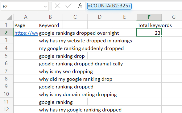
For example, I need to count the number of keywords my page ranks for. So, I enter "=COUNTA(B2:B25)" in a separate cell, where B2:B25 is the range of cells containing the keyword. The next thing I see is:
COUNTIF – to count the number of cells that meet certain criteria
Formula: =COUNTIF(range, criteria)
SEO use cases:
- Checking data consistency. You can check the consistency of your data across different cells or sheets. For instance, you can count the number of times a certain value appears in a column or check the number of duplicate entries.
- Evaluating performance. You can track the performance of your web pages or backlinks over time. For example, you can count the number of visits, clicks, or conversions for a specific period and compare it to previous periods.
How-to:
- Select the cell and enter the COUNTIF formula in it.
- Inside the formula, specify the range of cells that you want to count and the criteria that you want to apply.
- Press Enter to display the number of cells that meet the criteria.
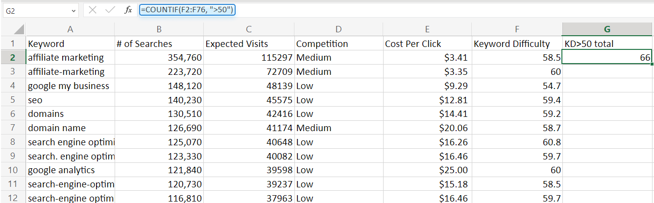
For example, I need to count the number of keywords with the keyword difficulty (KD) score higher than 50. So, I type "=COUNTIF(F2:F76, ">50")" in the cell where I want to see the result. Here, where F2:F76 is the range of cells containing the KD metric and “>50” is the condition for a high-difficulty keyword. The formula will display the number of keywords that meet the criterion.
Note
Use COUNTIFS to apply criteria to cells across multiple ranges and count the number of times all criteria are met. Its syntax is =COUNTIFS(criteria_range1, criteria1, [criteria_range2, criteria2]…)
SUM – to calculate the total for some metric
Formula: =SUM(number1, [number2], ...)
SEO use cases:
- Calculating metrics and analyzing data. You can calculate various SEO metrics such as total organic traffic, backlinks, or social media shares. By doing this, you evaluate the overall performance of your website or individual pages.
- Budgeting and forecasting. Use the SUM function to calculate budgets and create forecasts for your SEO campaigns. For example, calculate the total cost of your PPC campaigns or estimate the potential ROI of your content marketing efforts.
How-to:
- Select the cell where you want to display the result and enter the SUM formula in it.
- Inside the formula, type the numbers or cells that you want to add up, separated by commas.
- Press Enter.
For example, I need to calculate the total clicks for a set of keywords. So, I go to my spreadsheet and enter "=SUM(B2:B21)" in a separate cell. Here, B2:B21 is the range of cells containing the number of clicks for each of my keywords.
SUMIF – to add up a series of values that meet a certain criterion
Formula: =SUMIF(range, criteria, [sum_range])
SEO use cases:
- Analyzing traffic data. With the formula, you can calculate the total traffic for a specific keyword or landing page. It will help you identify the most popular pages on your website or track the performance of your SEO campaigns.
- Checking link quality. You can count the number of backlinks from high-quality domains. Later you can evaluate the link profile of your website.
- Comparing data sets. You can use the SUMIF function to compare data sets from different sources or periods. For instance, you can calculate the total search volume for a set of keywords and compare it to previous periods or competitors' data.
How-to:
- Select the cell and enter the SUMIF formula.
- Inside the formula, specify the range of cells that you want to evaluate, the criterion that you want to apply, and the range of cells that you want to add up.
- Press Enter to see the total sum.
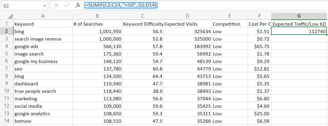
For example, I want to calculate the total expected traffic for a set of low-difficulty keywords. So, I enter "=SUMIF(C2:C139, "<50", D2:D139)" in a separate cell. Here, C2:C139 is the range of cells containing the keyword difficulty, "<50" is the criterion for low keyword difficulty, and B1:B139 is the range of cells containing the expected traffic data for each page.
Note
Traditionally, you can use SUMIFS to sum cells in a range that meets more than one criterion. The syntax is as follows: =SUMIFS(sum_range, criteria_range1, criteria1, [criteria_range2, criteria2], ...).
XLOOKUP – for matching data between different tables
Formula: =XLOOKUP(lookup_value, lookup_array, return_array, [if_not_found], [match_mode], [search_mode])
SEO use cases:
- Researching keywords. With the formula, you can search for a specific keyword in a large dataset and retrieve associated information such as search volume, competition, and estimated CPC.
- Analyzing competition. For instance, you can compare different websites or pages based on specific metrics such as domain authority, page authority, or backlink count.
- Analyzing content. You can retrieve data about your content such as word count, readability score, or keyword density, and compare it to similar content from competitors or high-ranking pages.
How-to:
- Select the cell where you want to display the result and enter the XLOOKUP formula in it.
- Inside the formula, specify the lookup value that you want to search for, the array where Excel should search for the lookup value, and the return array where Excel should retrieve the associated information.
- Press Enter.
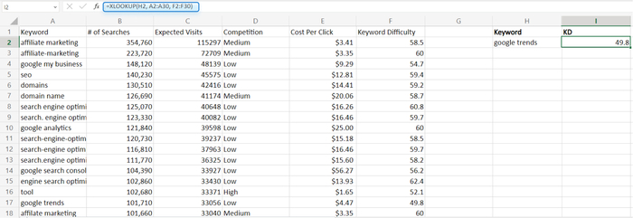
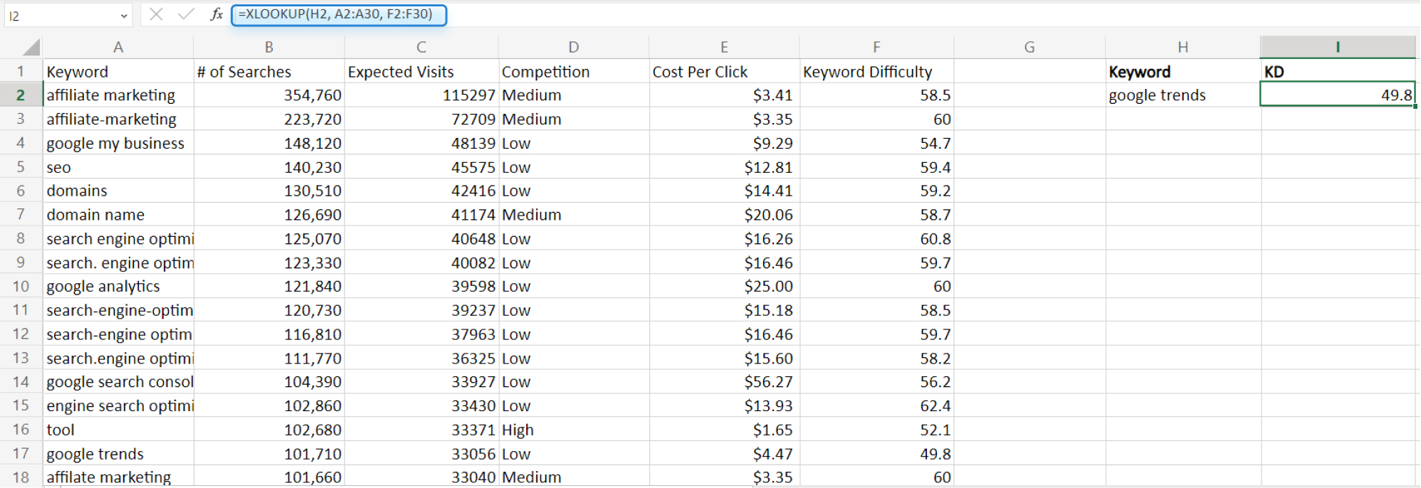
Say I want to retrieve the keyword difficulty of a specific keyword from a table that contains multiple columns of data. So, I use the following formula: =XLOOKUP(H2, A2:A30, F2:F30). Here, H2 is the keyword cell you analyze (your lookup value), A2:A30 is the lookup array that contains the keywords, and F2:F30 is the range where Excel will get the associated info from.
MAX and MIN – to find the highest and the lowest value in a range of data
Formula: =MAX(number1, [number2], ...) or MIN(number1, [number2], ...)
Use cases in SEO:
- Analyzing website performance metrics. You can find the highest and the lowest bounce rate, page load time, or exit rate among your website pages. This info will help you identify areas for improvement and optimization.
- Comparing keyword rankings. You can find the highest and the lowest keyword ranking positions among different search engines or over a specified time period. This way, you can track and improve your search engine visibility.
- Analyzing content engagement. You can find the highest and the lowest number of shares, likes, or comments for a piece of content. This can help you gauge the popularity and engagement of your content among your target audience.
How-to:
- Select the cell and enter the MAX or MIN formula in it.
- Inside the formula, specify the range of cells that you want to find the highest/lowest value for.
- Press Enter to see the result.
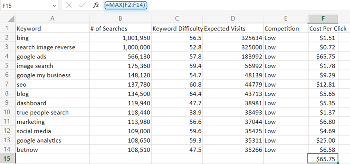
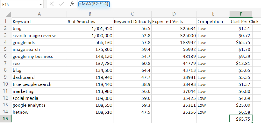
For instance, I want to find the highest СPС among my site keywords. In my spreadsheet, I enter "=MAX(F2:F14)" in a separate cell, where F2:F14 is the range of cells containing the CPC data.
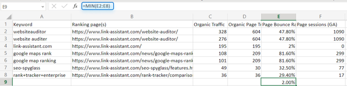
In the same way, if I need to find the lowest bounce rate among my website pages, I enter "=MIN(E2:E8)" in a separate cell, where E2:E8 is the range of cells containing the bounce rate data.
FAQ
Google Sheets and Excel are pretty much the same in terms of formula syntax. It means you can use many Excel formulas in Google Sheets with little or no modification.
However, there are some Excel-specific functions and formulas that are not available in Google Sheets, and some Excel formulas may produce slightly different results in Google Sheets due to differences in how the two programs handle certain calculations.
If you are familiar with Excel formulas and switching to Google Sheets, it's a good idea to test your existing formulas to make sure they work as expected.
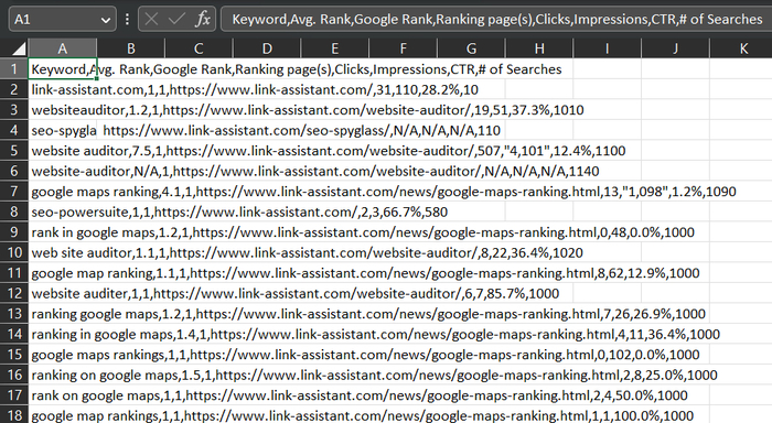
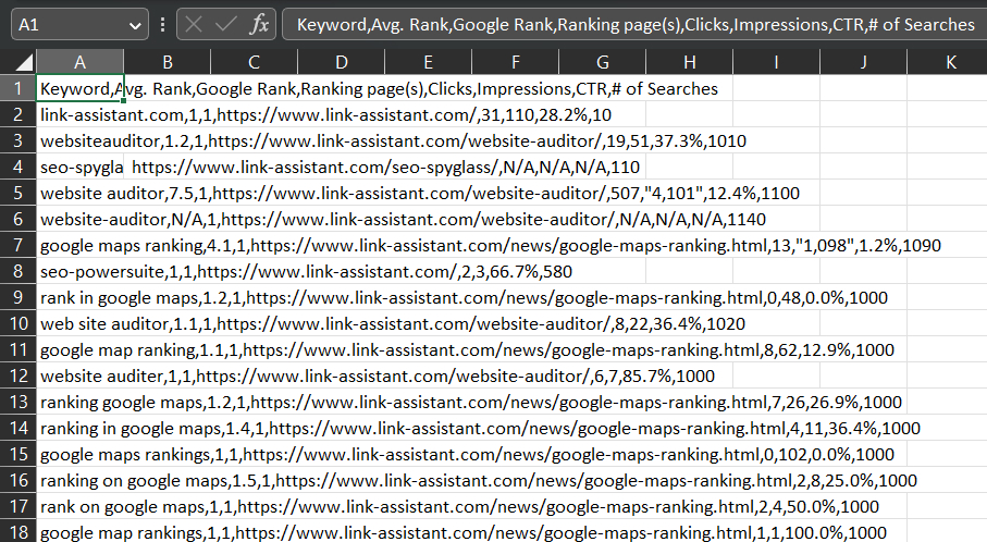
When you export your data from tools like SEO Powersuite and then open the file via Excel, you may see the following:
It’s not readable or manageable. What you need to do is:
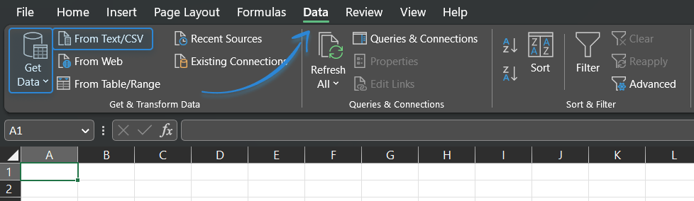
1. Open a new Excel workbook, go to the Data tab in the ribbon and click Get Data From Text/CSV.
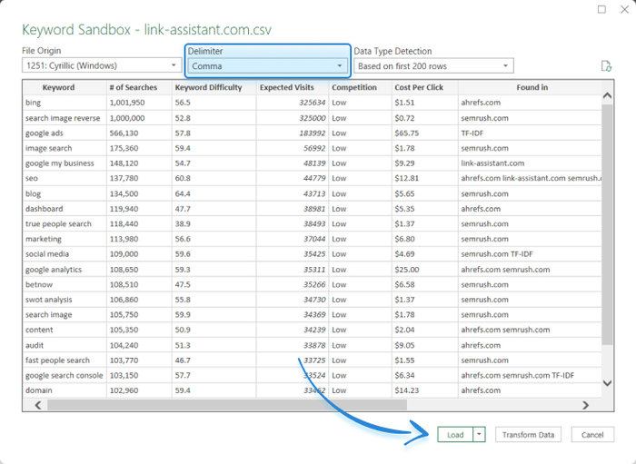
2. Select the needed file and in the popup window choose comma as a delimiter.
3. Click Load to see well-presented data.
Alternatively, you can learn how to import data correctly so that you don’t have to bother yourself with the delimiter change.
Yes, Excel provides a feature called "AutoFill" that allows you to quickly apply a formula to a large dataset.
You can simply enter the formula in the first cell, select the cell, and then drag the fill handle (a small square in the bottom-right corner of the selected cell) across the range you want to apply the formula to. Excel will automatically adjust the references in the formula for each corresponding cell in the range.
Or, it’s even easier if you want to apply the formula for the whole column: just hover over the bottom left corner of the sell til the black + sign appears and then double click. Your formula will be immediately applied to all the cels in the column.
Absolutely! Excel allows you to nest formulas within each other to perform more advanced calculations. For example, you can use the output of one formula as the input for another formula. By combining formulas, you can create powerful and flexible calculations to analyze and manipulate your SEO data.
For example, with the SUBSTITUTE function, you cannot replace more than one string at a time. However, you can nest one SUBSTITUTE inside another like this: =SUBSTITUTE(SUBSTITUTE(A1, “something to replace”, “something to replace with”), “something to replace 2”, “something to replace with 2”)
In fact, you can nest up to 64 levels of functions in a formula.